Look at that! Brain volume and surface visualization with Connectome Workbench's wb_view

Detailed anatomical investigations of the brain can greatly benefit from studying both a brain scan itself, i.e. the three-dimensional volume representation, and of the brain surface, i.e. the two-dimensional cortical mesh. In a previous post, I mentioned some of the commonly used image viewers, but here I would like to go into more detail about Connectome Workbench’s visualization software wb_view. Basic usage of wb_view is well documented in the official online tutorial, but I started using some advanced features that I would like to share with you.

Below, I show examples using data that was kindly provided by the Human Connectome Project, WU-Minn Consortium (Principal Investigators: David Van Essen and Kamil Ugurbil; 1U54MH091657) funded by the 16 NIH Institutes and Centers that support the NIH Blueprint for Neuroscience Research; and by the McDonnell Center for Systems Neuroscience at Washington University.

Clipping box

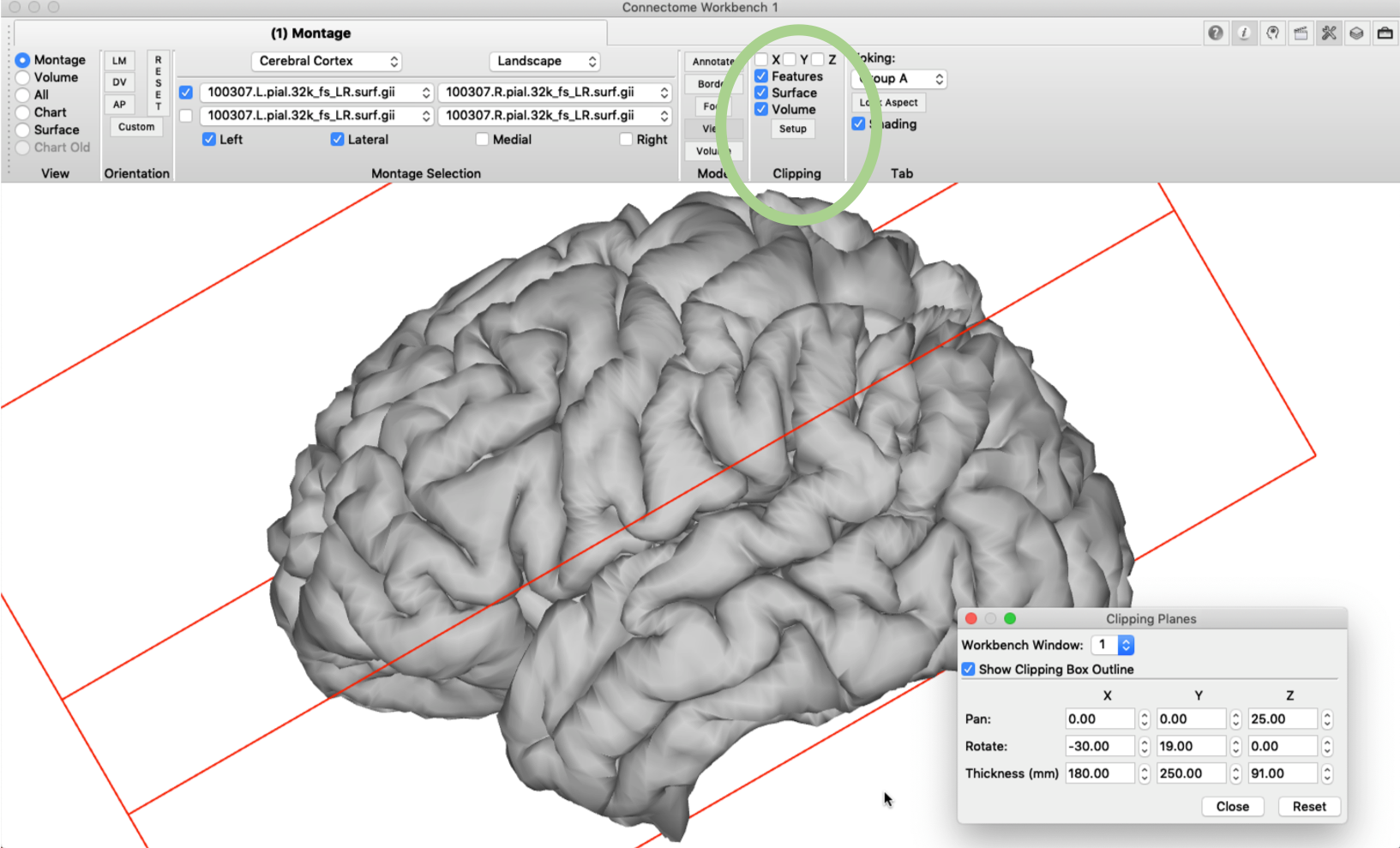
Some parts of the cortex, such as the insula or the opercular cortex, can’t be directly observed on the pial surface (hence the name for operculum = cover lat.). The ‘clipping box’ option, however, gives us the opportunity to make a virtual cut through the brain using a plane with user-specified orientation. This ‘cut’ can also be used to visualize a slice of arbitrary orientation in a brain volume, as described further below. Settings for the clipping box can be edited in the ‘Clipping’ pane under ‘Setup’. In the example below I changed the settings so that the temporal lobe falls outside the box. Next, we tick the ‘Z’ box in the Clipping pane and the cut will be performed along the z-dimension of the box.

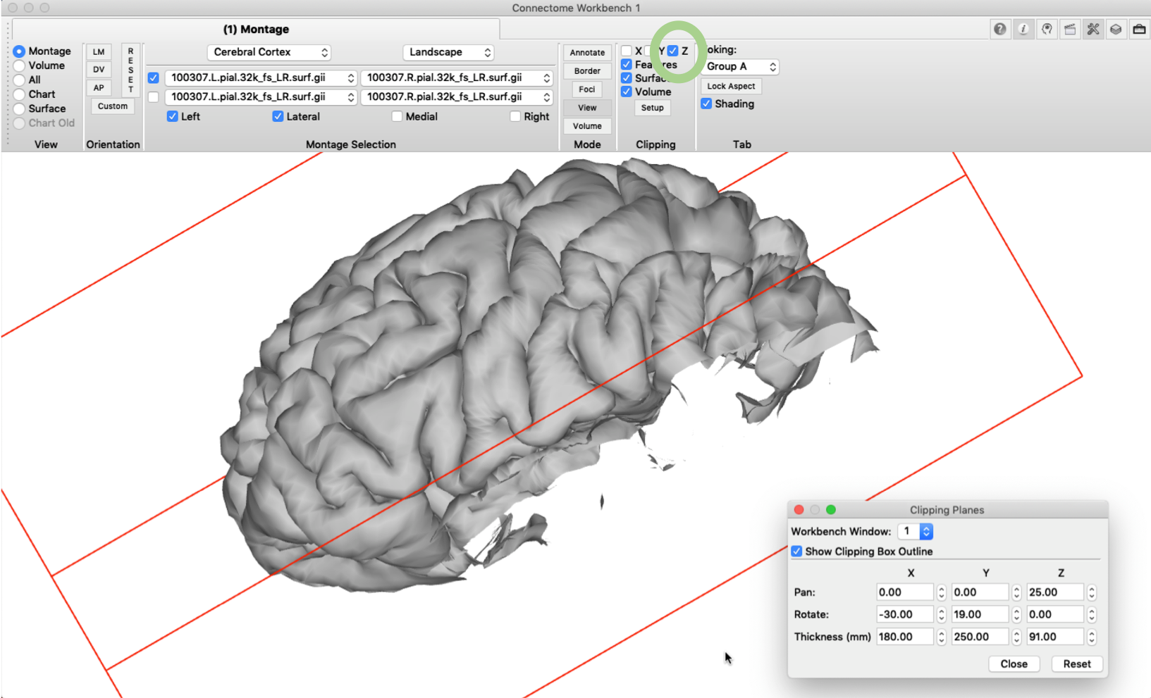
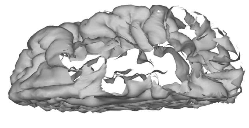
If we then rotate the brain surface, we are able to inspect the opercular cortex without having the temporal lobe in the way.

Tile Tabs

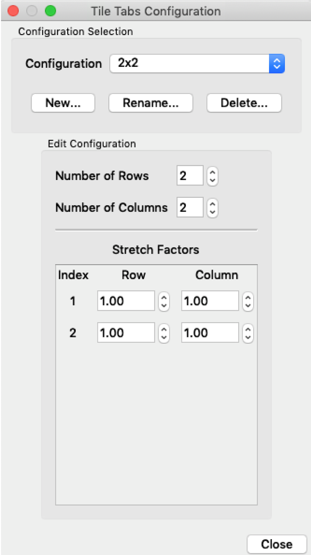
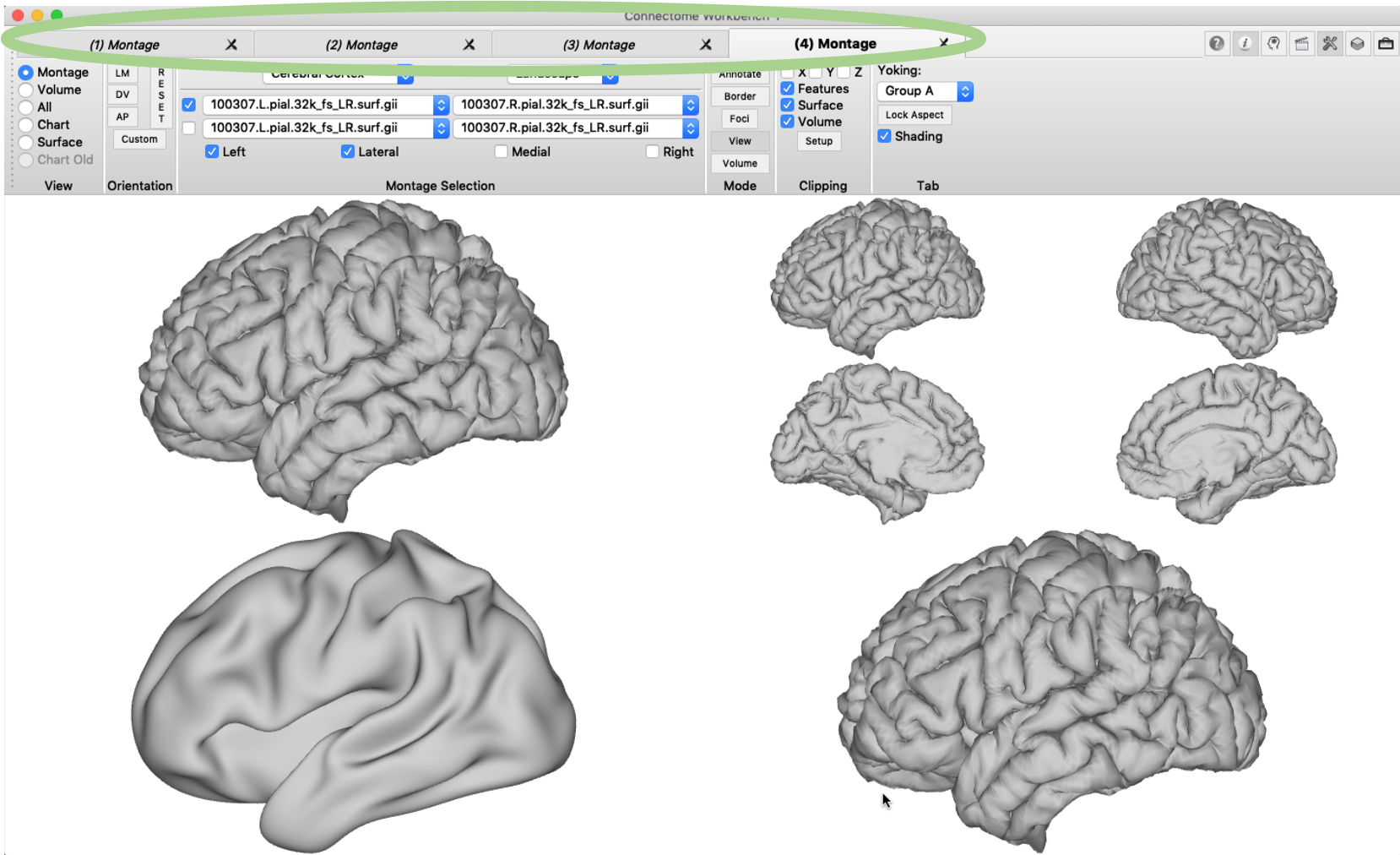
Tile tabs will help you to produce a neat arrangement of subfigures that can be directly turned into a manuscript figure. First, the configuration of the figure matrix (e.g. 2 by 2) needs to be specified. You will find the menu in ‘View’ -> ‘Tile Tabs Configuration’ -> ‘Create and Edit…’.

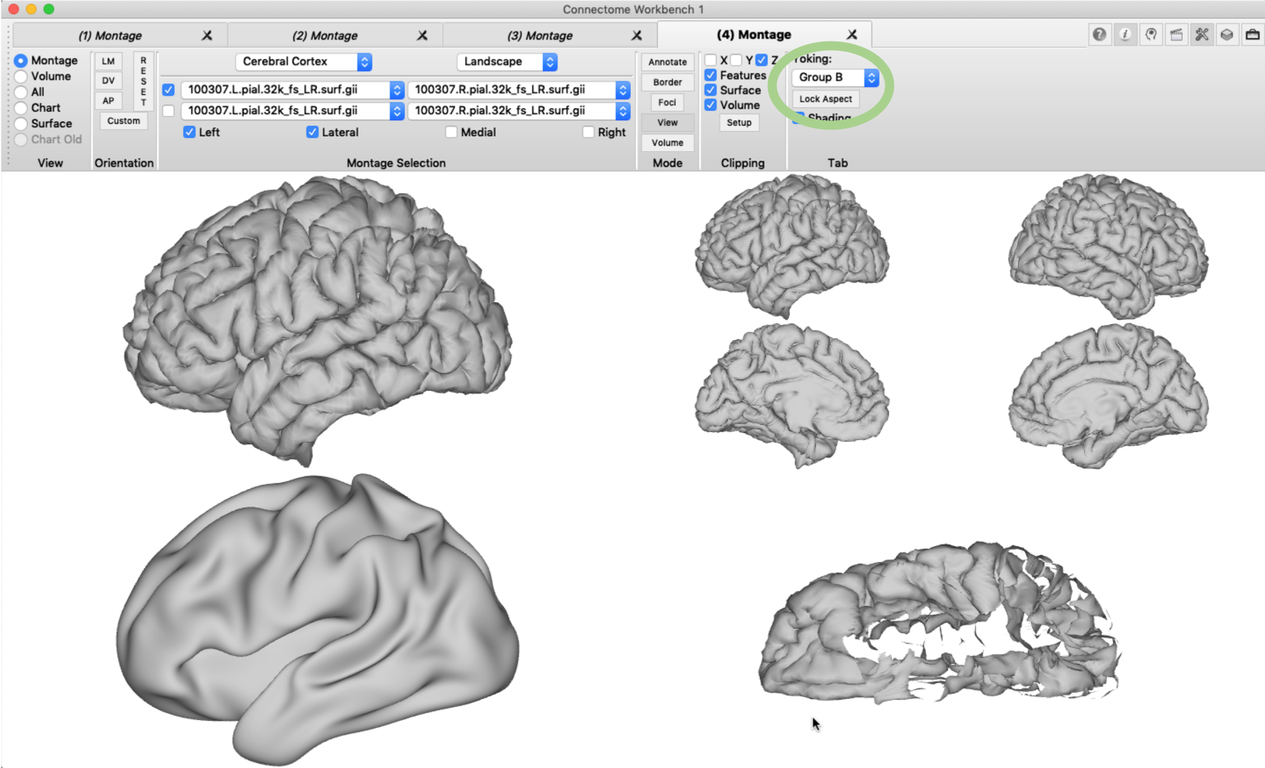
Next, the tile tabs display mode needs to be activating by clicking ‘View’ -> ‘Enter Tile Tabs’. The four required tabs are not directly produced, but up to three new tabs can now be added using ‘File’ -> ‘New Tab’ (or using the short-cut cmd+D). You can display different surfaces (.surf.gii) in each tab using the ‘Montage Selection’ pane, but only surfaces with the same number of vertices can be loaded at the same time. In the example below, I loaded in addition a right pial surface and a left inflated brain surface. You will notice that by default the surfaces in tile tabs are ‘tied’ together, i.e. when you change the orientation of one of them, all the others will change accordingly. This is called ‘yorking’ and it can be changed in the ‘Tab’ pane. In the example below, I chose a different yorking-group for the last tile tab, enabled the clipping box and rotated the surface.

View a volume file in arbitrary orientation

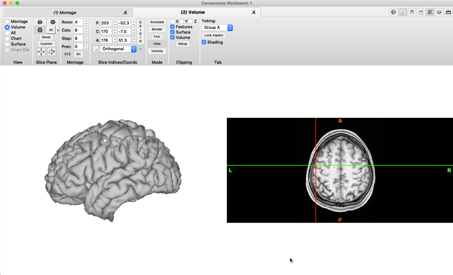
Tile tabs are very useful when it comes to viewing a brain surface and a 3D brain scan at the same time. You can load a nifti file into wb_view and display it in a tab by ticking ‘Volume’ in the ‘View’ pane. When you select a specific vertex in the brain surface (see the grey dot below), the cursor in the volume tab will jump directly to the corresponding voxel.

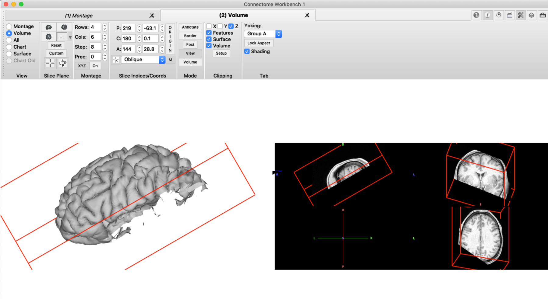
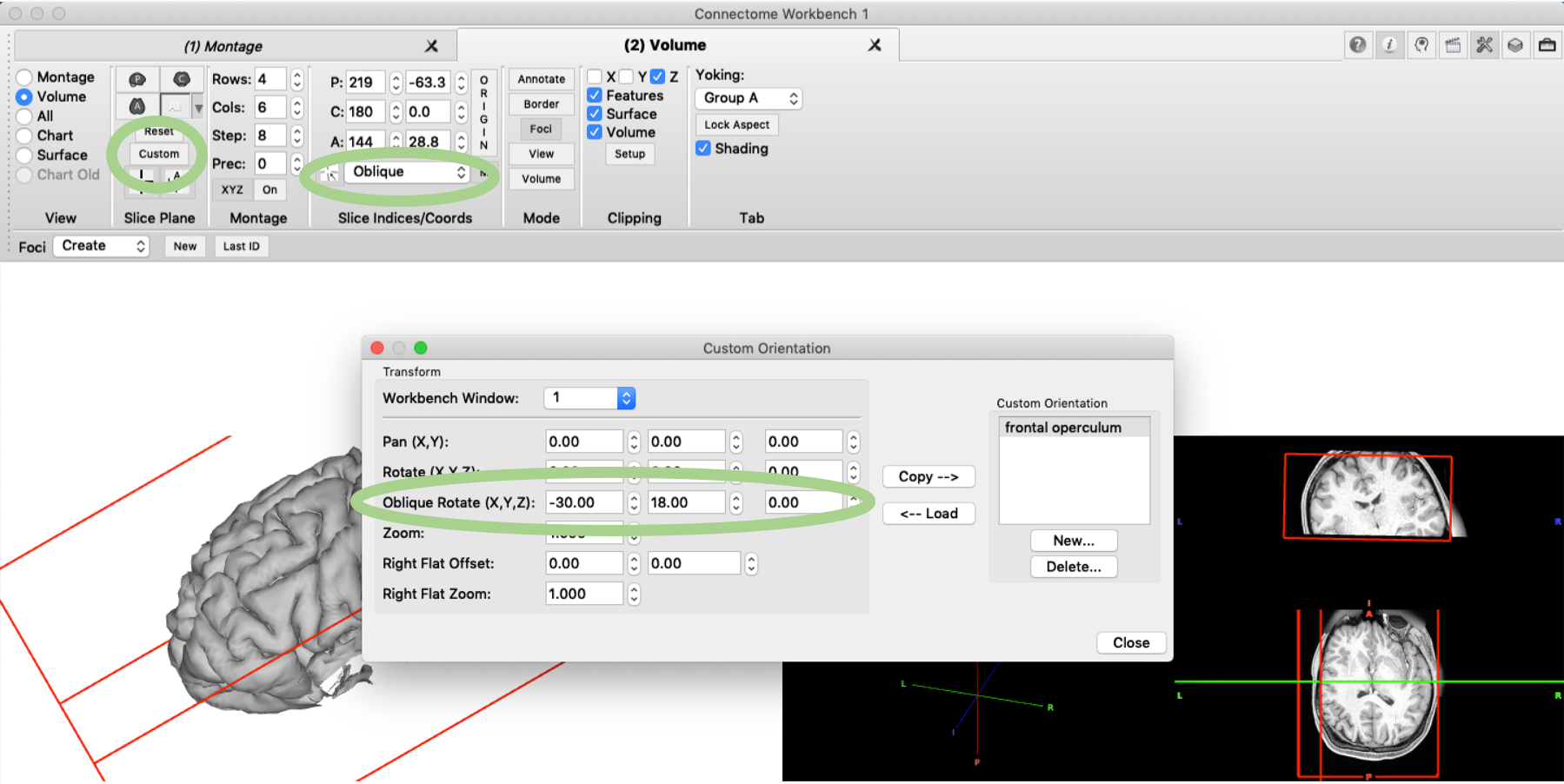
As mentioned above, the clipping box can be also applied to volume data (if ‘Volume’ is ticked in the ‘Clipping’ pane). The brain volume can then be rotated accordingly so that the brain slice of the cut will be visible. First, the rotation needs to be enabled by changing the setting in the ‘Slice Indices’ pane from ‘orthogonal’ to ‘oblique’. The exact rotation can then be set in the ‘Slice Plane’ pane under ‘Custom’. As XYZ coordinates for the oblique rotation, we enter the same values that we used for the clipping box itself. This orientation can also be saved so that it can be reloaded in another session.

Foci from XYZ coordinate

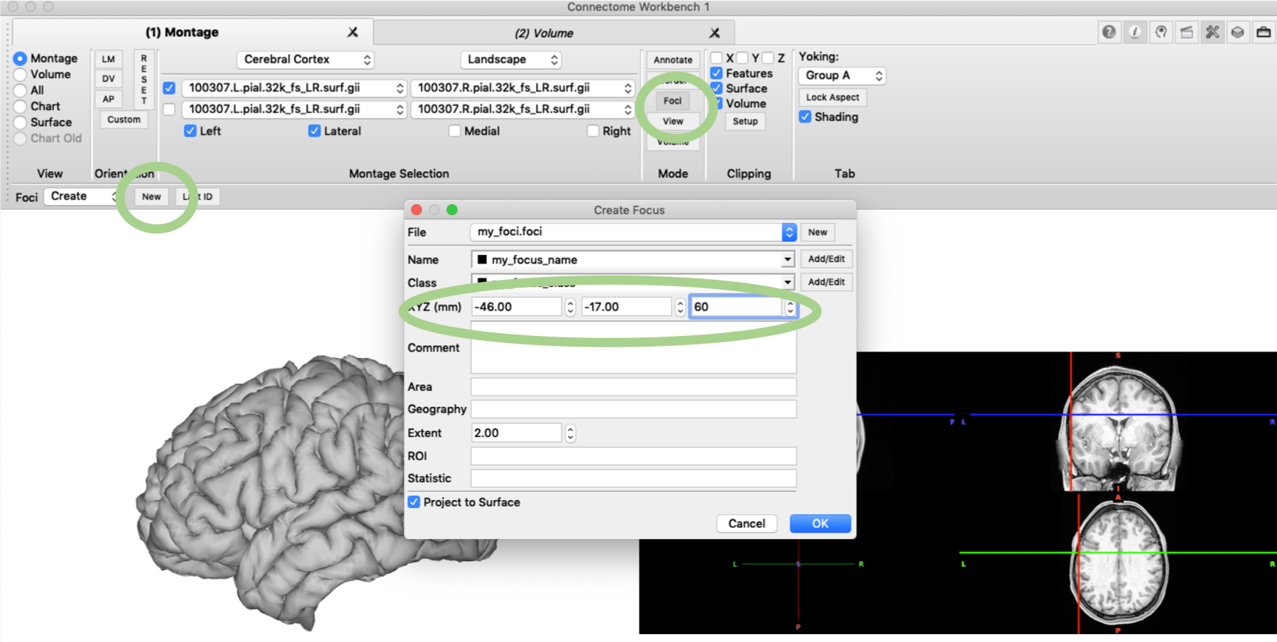
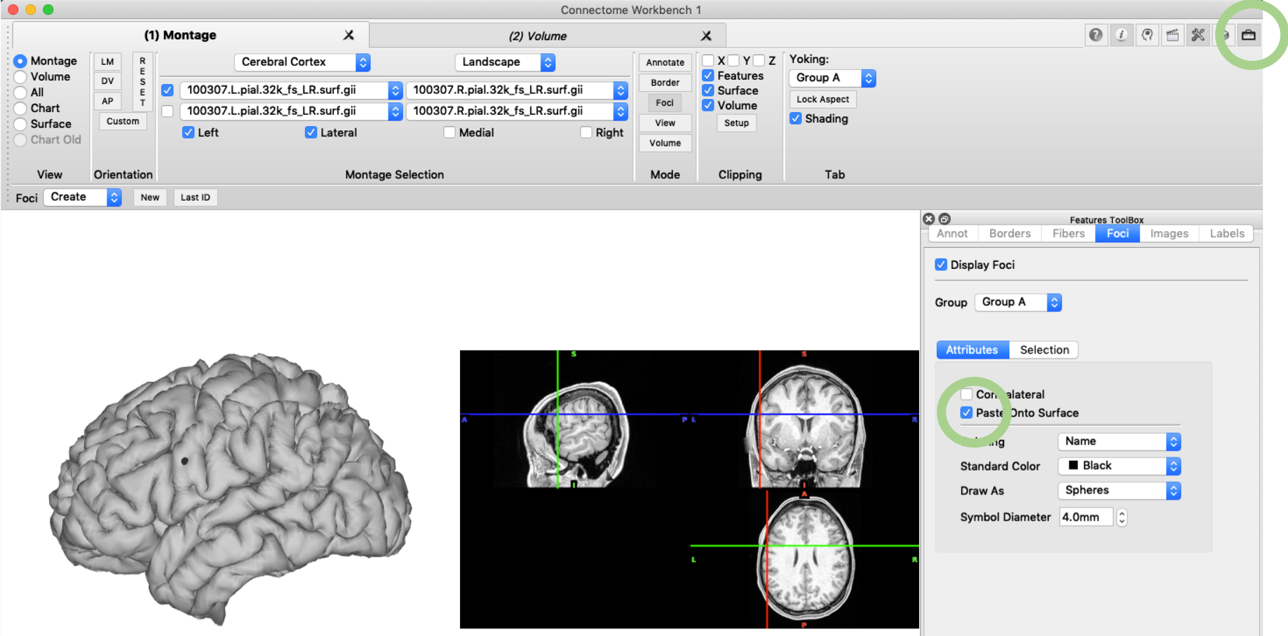
Another feature that can be very useful to create a nice manuscript figure are foci, i.e. focal highlights on the brain surface. You can create such a focus in the ‘Mode’ pane under ‘Foci’ and then ‘Create’ ‘New’. In the pop-up menu you can specify the XYZ coordinates and set the file name as required. Display of the Foci can be enabled in the ‘Features Toolbox’ and you might want to use ‘paste onto surface’.

Automated scene file creation

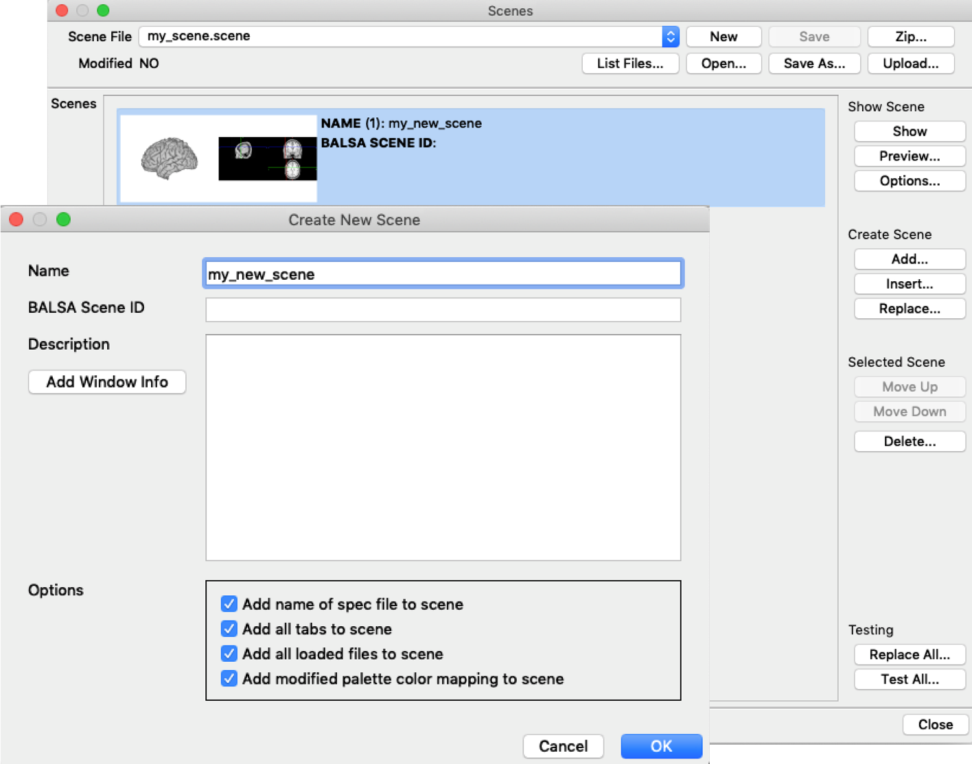
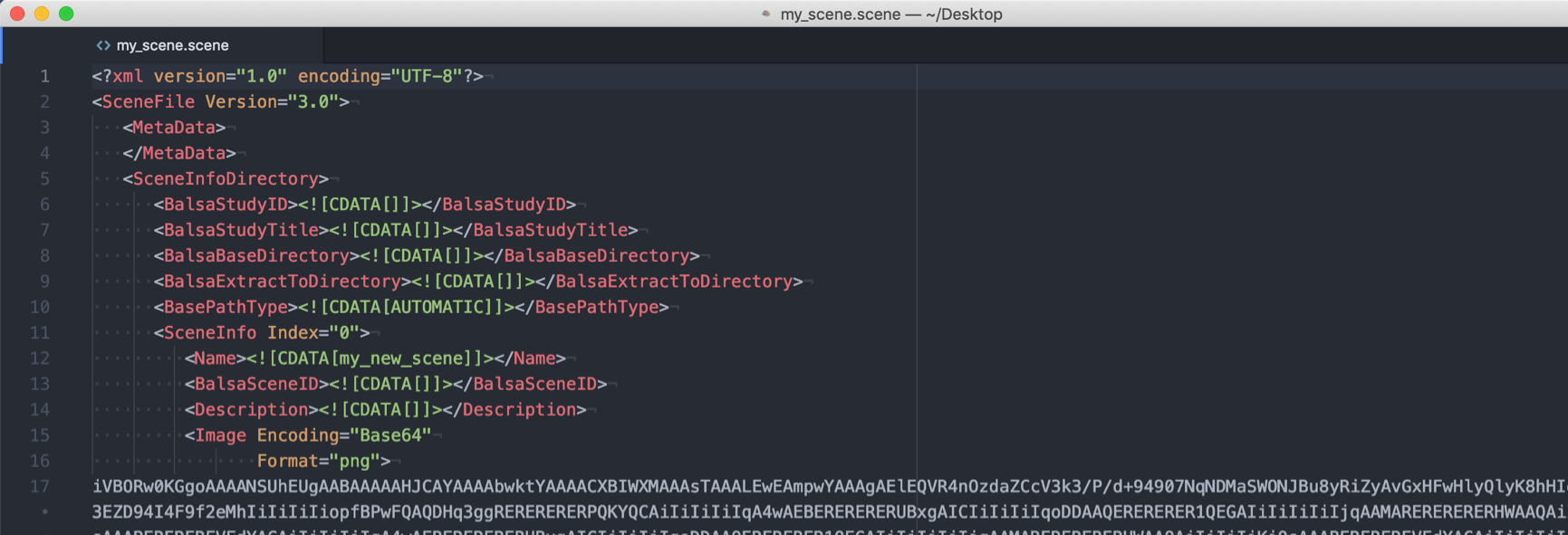
When you’re done with setting up you wb_view visualization, you can continue to store the whole display configuration using a so called ‘scene’. You can create a scene file, which can store multiple scenes, in ‘Window’ -> ‘Scenes’ (or by clicking the Scenes icon). When you click ‘Create Scene’ ‘add’, you can decide if you want to include all loaded files, tiles, etc. with the current scene. You might consider unticking some boxes, because a large scene file can take a long time to load. Don’t forget to create the actual scene file (my_scene.scene) in the top of the window and save everything.

Now imagine you spent all this time creating a scene file using data from an individual subject, wouldn’t it be great if you could automatically reproduce the same scene for another subject? This is possible, if all required files can be accessed with the identical file paths that only differ in subject-ID. In order to turn the scene file into a script, first load it into an editor, for example atom.

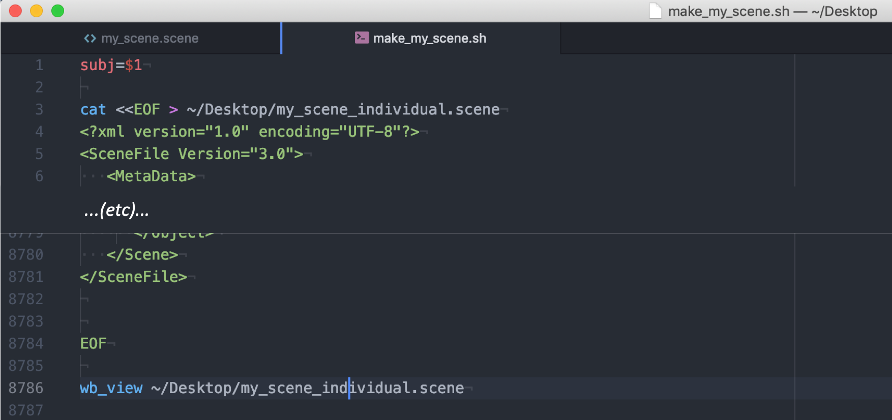
Then add two lines on the top of the file to parse the command line argument for the subject ID and to write out a new scene file. At the bottom of the script, close the EOF section and load the new scene file into wb_view.

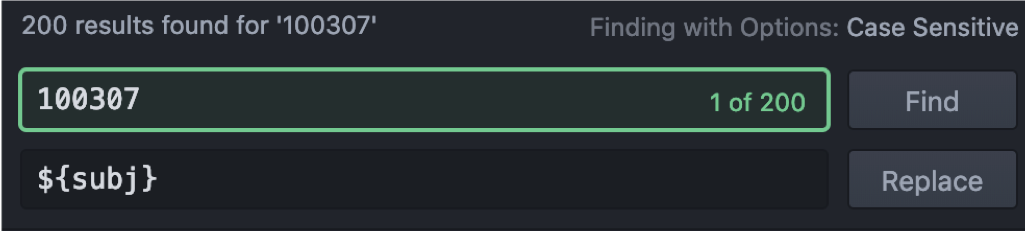
The subject-ID (here 100307) needs to be replaced by ‘${subj}’ throughout the file. Save the new file as script with the ending ‘.sh’.

When we call this script from the command line, it will now automatically create the scene file for the subject with the ID that we provide in the call:

wb_view ~/Desktop/my_scene_individual.sh 106452

That’s it!

These were just a few examples that I found worth detailing beyond the level that I found in the online tutorial. However, wb_view provides much more functionality for displaying overlays, making annotation, etc., so this is just the tip of the iceberg. I hope these tips were helpful and will make your surface/volume visualization easier.

Thanks for reading this post :-)

Nicole