Getting your blobs: general linear model vs. machine learning

One of the criticism that the neuroimaging community faces is the supposedly misguided obsession to find ‘blobs’ in the brain that ‘light up’ when a persons performs a cognitive task. Some of the criticism is turned towards the interpretation of questionable topics (for example “which brain area controls love?”), other people see the issue in experimental design or statistical analysis (limited power, p-hacking, etc.). Here, I don’t want to discuss the pros and cons of fMRI, but I rather want to demonstrate alternative methods to obtain statistical maps, which highlight a brain area where an effect is present.

Example case to test

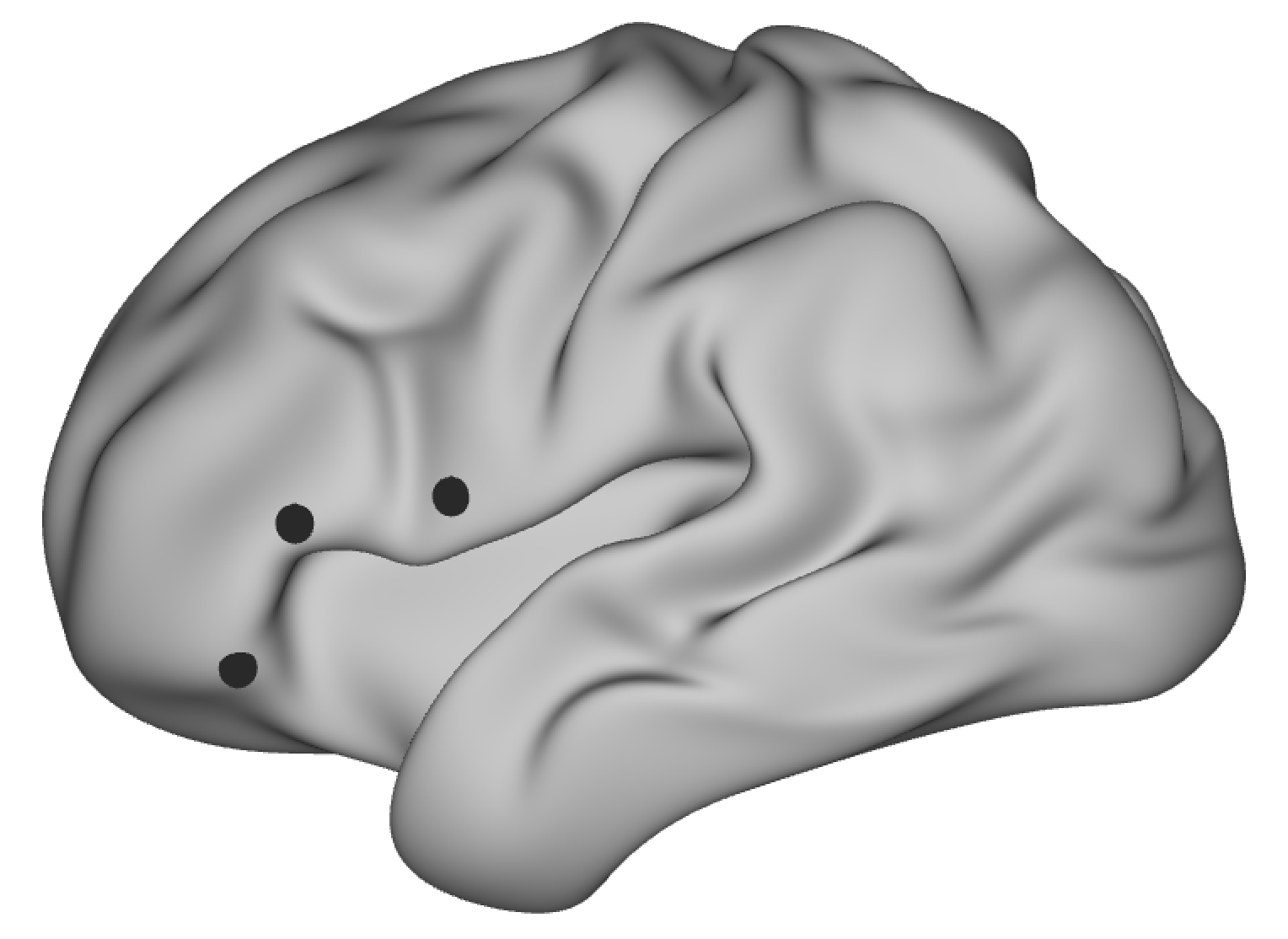
As example, I’m comparing functional connectivity maps of three brain areas in left inferior frontal cortex. This is not a task-based question, but similar analysis methods can be used in this context. I selected three foci on a standard surface in wb_view, roughly based on three different anatomical brain areas. The underlying surface patch was transformed to volume space and then I derived seed-based correlation maps on the cleaned resting-state data using FSL tools. The correlation maps are used as a proxy of functional connectivity between the seed voxels and the rest of the brain. The code for these processing steps (in Shell script) is shown below. Data were provided by the Human Connectome Project, WU-Minn Consortium (Principal Investigators: David Van Essen and Kamil Ugurbil; 1U54MH091657) funded by the 16 NIH Institutes and Centers that support the NIH Blueprint for Neuroscience Research; and by the McDonnell Center for Systems Neuroscience at Washington University. All result maps are overlaid onto the MNI standard template.

mydir=/my_path/
HCPdir=/path_to_HCP_subjects_data/
# file that contains 3 foci drawn on standard surface
foci=$mydir/seeds.foci
# hemisphere
hemi=L

sub_list='01 02 03 04 05 06 07 08 09 10 11 12 13 14 15 16 17 18 19 20'
# list of foci in foci-file
seed_list='broca1 broca2 broca3'
for seed in $seed_list; do
    for sub in $sub_list; do
        # subject's data processed using HCP-pipeline
        DD=$HCPdir/${sub}/MNINonLinear
        # surface with vertex-correspondance to standard surface
        surface=$DD/MNINonLinear/${sub}.${hemi}.pial.164k_fs_LR.surf.gii
        # 4D resting-state fMRI scan from
        rest_scan=$DD/func/rest/rest.ica/filtered_func_data_clean_standard.nii.gz
        # name of output for surface seed
        seed_surf=$mydir/${sub}_${seed}_seed.func.gii
        # name of output for volume seed
        seed_vol=$mydir/${sub}_${seed}_seed.nii.gz
        # name for seed-based correlation map
        sbcm=$mydir/${sub}_${seed}_sbcm

        # get the vertex that is underlying the foci
        echo 'get vertex from foci'
        wb_command -foci-get-projection-vertex $foci $surface $seed_surf -name $seed

        # smooth and binarize around the vertex to get circular patch
        echo "smooth"
        wb_command -metric-smoothing $surface $seed_surf 1 $seed_surf
        wb_command -metric-math "(x>0)" $seed_surf -var x $seed_surf

        # project the surface patch to the subject's resting state volume space
        echo 'project vertex to volume'
        wb_command -metric-to-volume-mapping $seed_surf $surface $rest_scan $seed_vol -nearest-vertex 3

        # compute seed-based correlation map
        echo 'get SBCM'
        fsl_sbca -i $rest_scan -s $GD/MNI152_T1_24mm_brain_mask.nii.gz -t $seed_vol -o $sbcm

        echo 'convert to z-maps'
        fslmaths ${sbcm}_corr.nii.gz -sub `fslstats ${sbcm}_corr.nii.gz -M` -div `fslstats ${sbcm}_corr -S` ${sbcm}_corr.nii.gz
        fslmaths ${sbcm}_corr -mas $GD/MNI152_T1_24mm_brain_mask.nii.gz ${sbcm}_corr
    done
done

# merge all subjects' maps into one 4D file
merged_maps=$mydir/merged.nii.gz

# initialize file with subject-blocks information
> $mydir/blocks.csv
# loop over seeds
for seed in $seed_list; do
    ind=1
    # make average map for each seed
    fsladd $mydir/${seed}_sbcm_avg.nii.gz -m $mydir/*_${seed}_sbcm_corr.nii.gz
    # initialize string for filenames to be added
    cmd_str=""
    for sub in $sub_list; do
        echo "add $sub $seed"
        # add subjects z-stats map to merged_maps
        cmd_str="$cmd_str $mydir/${sub}_${seed}_sbcm_corr.nii.gz"
        # add subject number to subject-blocks information
        echo $ind >> $mydir/blocks.csv
        # increase count
        ind=$(( $ind + 1))
    done
done
fslmerge -t $merged_maps $cmd_str

General linear model approach

A general linear model (GLM) can be thought of as an extension of a linear regression, where we specify a statistical model. Then we test for each voxel, how well it fits the model and save the statistical value associated with the test. All these voxel-wise values result in a statistical image, that can be thresholded so that only the parts of the brain that fit our hypothesis (significantly) well are highlighted. There are various softwares to implement a GLM-based analysis and here I used PALM similar as described in a previous post. For this example, let’s say we are not interested in a single contrast of how the connectivity for two of the areas differ, but rather in the brain areas that are generally sensitive to which one of the three seeds we use. This corresponds to an f-test over the three possible contrasts (area1 vs area2, area2 vs area3, area1 vs area3). The code below (in Python) shows how I set up the GLM and then call PALM.

import numpy as np
import os
import sys
import matplotlib.pyplot as plt

# define file names
target = os.path.join(mydir, 'merged.nii.gz')
out_glm = os.path.join(mydir, 'my_glm.csv')
out_con = os.path.join(mydir, 'my_con.csv')
out_f = os.path.join(mydir, 'my_f.csv')
out_palm = os.path.join(mydir, 'glm')

factor = ['broca1', 'broca2', 'broca3']
n_subs = 20

# EVs
col_factor1 = np.array([1, 0, 0]).repeat(n_subs).reshape(-1, 1)
col_factor2 = np.array([-1, 1, -1]).repeat(n_subs).reshape(-1, 1)
col_factor3 = np.array([-1, -1, 1]).repeat(n_subs).reshape(-1, 1)

# random effects term for participants (stack 3 times)
col_ppt = np.vstack((np.identity(n_subs), np.identity(n_subs), np.identity(n_subs)))

# combine all columns into a design matrix
my_glm = np.hstack((col_factor1, col_factor2, col_factor3, col_ppt))

# check if shape makes sense
print(my_glm.shape)
# plot GLM
# plt.imshow(my_glm, aspect='auto')
# plt.show()

# set up contrasts
n_effects = 3
n_contrasts = 3
my_con = np.zeros([n_contrasts, my_glm.shape[1]])
my_con[:, 0:n_effects] = np.array([[1, 0, -1],
                                    [0, 1, -1],
                                    [0, 0, -1]])

# set up f-test
my_f = np.array([[1, 1, 1]])

# write out design, contrast and f-test as files
np.savetxt(out_glm, my_glm, fmt='%1.0f', delimiter=",")
np.savetxt(out_con, my_con, fmt='%1.0f', delimiter=",")
np.savetxt(out_f, my_f, fmt='%1.0f', delimiter=",")

print('run PALM')
n_permutations = 5000
palm_command = (f"palm -i {target} -d {out_glm}  -t {out_con} -f {out_f} -o {out_palm} -n {str(n_permutations)} -quiet -noniiclass -logp")
print(palm_command)
os.system(palm_command)

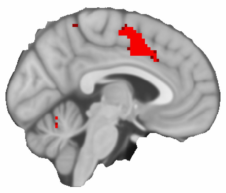
The analysis above produces a statistical image for each of the three contrasts that we specified, but also for the f-test, which indicates where the means of all three correlation maps are different. Below you see how the resulting map of p-values for an example brain slice. I’m not going to interpret the result, because I use this just as an example of how to perform this analysis and how a possible output can look like. More careful considerations about the seed-placement and data processing are required to get a robust and interpretable result.

Classifier sensitivity approach - get to know PyMVPA

A different way to address our question is to use a classifier as machine learning technique instead of a pre-defined statistical model. There are many papers and blogs that address the pros and cons of both approaches and unfortunately, I can’t go into depth about the comparison here (and the title of this blog post might actually be misleading). I found the Python-based open-source toolbox PyMVPA a great resource to find out more about statistical learning analysis of neuroimaging data and most of the code below has been adapted from their tutorials.

As a first step, we need to load the data and bring it into the correct format together with the necessary information (ROI labels, subject IDs, etc.). Then we can define a classifier and set up a cross-validation procedure. The performance of the classifier on our dataset can be assessed using a confusion matrix. These steps are shown below for a simple k-nearest neighbour classifier.

import sys
import os
import numpy as np
from mvpa2.tutorial_suite import *
import matplotlib.pyplot as plt
from mvpa2.generators.partition import HalfPartitioner
from mvpa2.mappers.fx import mean_sample
from mvpa2.measures.searchlight import sphere_searchlight
from mvpa2.clfs.meta import FeatureSelectionClassifier
from mvpa2.measures.anova import OneWayAnova
from mvpa2.featsel.base import FractionTailSelector
from mvpa2.featsel.base import SensitivityBasedFeatureSelection
import nibabel as nib
import pickle

mydir = os.path.join('my_path')

# column containing subject ID's
subs = [line.rstrip() for line in open(os.path.join(mydir, 'blocks.csv'))]
# derive the number of unique subjects
n_subs = len(set(subs))
# ROI labels
x = ['broca1', 'broca2', 'broca3']
# make column of ROI labels for each row
targets = [item for item in x for i in range(n_subs)]

# group 5 subjects as 4 chunks
chunks = np.tile(np.array([1, 2, 3, 4]).repeat(5), 3)

# read in functional dataset
bold_fname = os.path.join(mydir, 'merged.nii.gz')
mask_fname = os.path.join(mydir, 'MNI152_T1_24mm_brain_mask.nii.gz')

print('read in ... : ', bold_fname)
ds = fmri_dataset(samples=bold_fname, targets=targets, chunks=chunks, mask=mask_fname)
print('done reading data')

# -----
# Get confusion matrix
# -----
print('Get confusion matrix...')
# set up classifier
clf = kNN(k=3, dfx=one_minus_correlation, voting='majority')
# set up cross-validation
cvte = CrossValidation(clf, NFoldPartitioner(attr='chunks'),
                       errorfx=lambda p, t: np.mean(p == t),
                       enable_ca=['stats'])
cv_results = cvte(ds)
# plot confusion matrix
print(cvte.ca.stats)
cvte.ca.stats.plot()
plt.show()

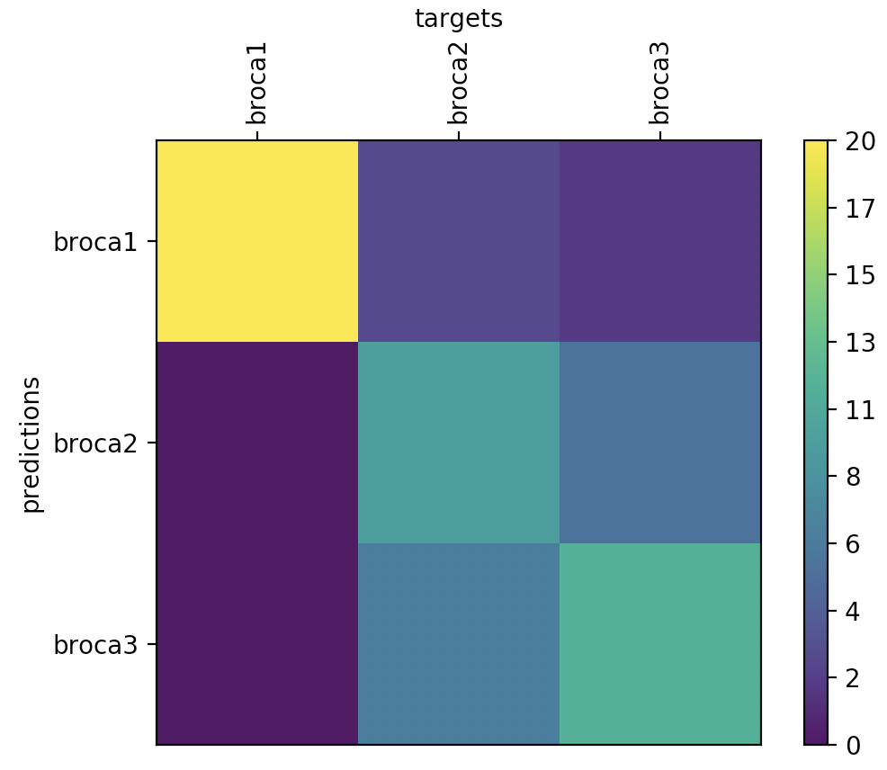
Well, the classification performance isn’t great, but keep in mind that we only provided data from 20 subjects, which is not even close to the recommendation for most statistical learning algorithms.

While the classifier performance can tell us something about how well this method could be use to predict the class of a novel correlation map, this is not very useful for our original question. We rather want to find out, which of the voxels differ between the three conditions and thereby inform the classifier. In order to localise, which parts of the brain are informative for the classifier, we can use a so called sensitivity analysis. This analysis provides a voxel-wise result for the three different contrasts. These sensitivity maps can be combined using a ‘maximal absolute value’ operation, which is somehow similar to an f-test as described above. The underlying code (using a support-vector machine this time) and the result are shown below:

# set up linear classifier
clf = LinearCSVMC()
# selects the most informative voxels based on top x% of one-way-ANOVA
fsel = SensitivityBasedFeatureSelection(OneWayAnova(), FractionTailSelector(0.05, mode='select', tail='upper'))
# feature selection classifier
fclf = FeatureSelectionClassifier(clf, fsel)
# cross-validation procedure
cvte = CrossValidation(fclf, HalfPartitioner())
# train classifier
fs_results = cvte(ds)
# set up sensitivity analyser
sensana = fclf.get_sensitivity_analyzer()
sens = sensana(ds)
# write out maps to nifti
sens_r = ds.a.mapper.reverse1(abs(sens.samples))
nimg = map2nifti(ds, sens_r)
nib.save(nimg, os.path.join(mydir, 'sensana.nii.gz'))

# combined f-test
sens_comb = sens.get_mapped(maxofabs_sample())
nimg_comb = map2nifti(ds, sens_comb)
nib.save(nimg_comb, os.path.join(mydir, 'sensana_comb.nii.gz'))

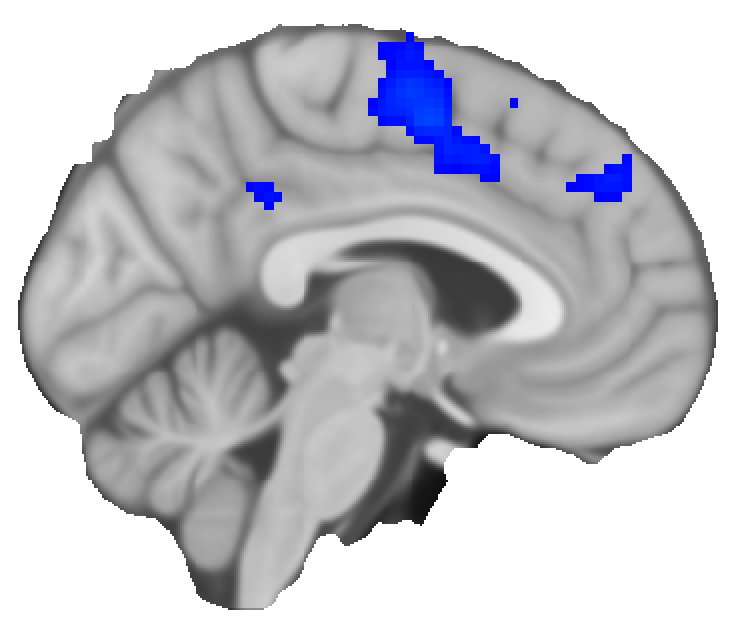
The result looks quite similar to the one from the GLM analysis, but I should point out that PALM takes several hours to run, while the sensitivity analysis runs almost instantaneously.

MVPA - The searchlight analysis

One downside of the two approaches described above, is that they are univariate methods that consider each voxel separately. For neuroimaging data, however, we know that the activation of each voxel’s local neighbourhood contains important information and the measurements are not independent. For this reason, multivariate (or multivoxel) pattern analysis (MVPA) has gained great popularity in the neuroimaging community. In MVPA, the underlying question is: Does the pattern of activations in this voxel’s neigbourhood encode information about the class?

One way of implementing MVPA for fMRI data is to use a ‘searchlight’ approach. Instead of a single voxel, we consider all voxels within a spherical ROI around the voxel jointly, which allows us to map the effect of local patterns. The implementation of the searlight analysis in PyMVPA is quite easy to use. In order to speed up the analysis, we can use a sensitivity analysis as described above to limit the search space of the sphere. This is an example snippet of how the searchlight analysis can be implemented in PyMVPA:

# set up classifier
clf = LinearCSVMC()
# # selects the most informative voxels based on top x% of one-way-ANOVA
fsel = SensitivityBasedFeatureSelection(OneWayAnova(), FractionTailSelector(0.05, mode='select', tail='upper'))
# feature selection classifier
fclf = FeatureSelectionClassifier(clf, fsel)
# cross-validation procedure
cvte = CrossValidation(fclf, HalfPartitioner())
# set up search light
sl = sphere_searchlight(cvte, radius=3, postproc=mean_sample())
res = sl(ds)
# wait....

# in which fraction of spheres is the error 2 SD lower than chance?
# compute errors
sphere_errors = res.samples[0]
res_mean = np.mean(res)
res_std = np.std(res)
chance_level = 1.0 - (1.0 / len(ds.uniquetargets))
frac_lower = np.round(np.mean(sphere_errors < chance_level - 2 * res_std), 3)
print(frac_lower)

# write out searchlight performance as nifti'
map2nifti(ds, 1.0 - sphere_errors).to_filename(os.path.join(mydir, 'sl.nii.gz'))

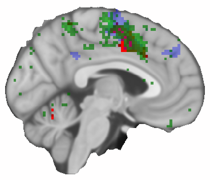
Above, is the result of the searchlight analysis (in green) shown together with the other two result maps. The most obvious difference to the previous figures is that the analysis seems to pick up more fine-grained details. But it also shows an effect further posterior, which was not picked up in the other two analysis approaches. It should be noted, however that the selection of the display threshold for the map might not be directly comparable.

What can we learn from this?

First of all, I should highlight again that the results shown above are (most likely) not a good representation of the differences in functional connectivity across different parts of left inferior frontal cortex. I selected the foci as illustrative example and other research groups have done much more careful work on this. Even more unsatisfactory, my conclusion of this post is that different analysis methods can lead to the same or different results. All of them have strengths and weaknesses, and your choice ultimately depend on your research question and underlying data (as always…).

But on a rather positive note, I wanted to demonstrate that the development of neuroimaging data analysis tools is a steadily growing and exciting field. All of the data and software used above is open-source and PALM and PyMVPA, for example, contain very well-documented UserGuides. I hope you can use the above explanations and code snippets as inspiration to try different analysis methods on your data to help your research.

That’s it

Thanks for reading this post :-)

Nicole