Many processing steps in the analysis of brain scans rely on an accurate alignment of images. For example, when I transform my results to a standard reference space or when I align a subject’s brain scans from multiple sessions or scanning modalities. Tools such as FSL’s¹ FLIRT automatically estimate a transformation that can map an input image to a reference. However, if my data is non-typical - for example from a different species or from neurological patients with brain lesions - I might not be satisfied with the result of the automatic estimation. But there is a solution: Thanks to linear algebra, we can manually adjust a transformation!

Here I’ll describe the theoretical background of this image manipulation, but you can find scripts that deal with it in my Github repository.

Let’s get started with some basics …

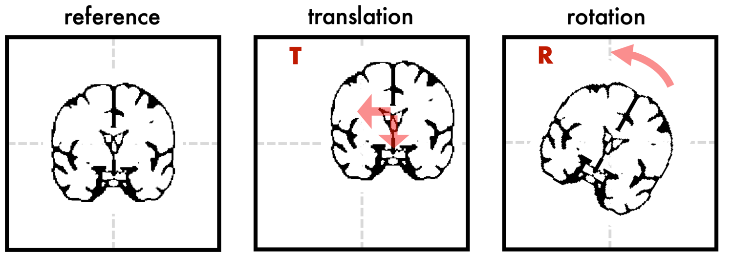
The type of transformation that I’m talking about is a ‘rigid body’ transformation. This means that the image can be translated (i.e. shifted) along the dimensions in space or rotated along the three spatial axes, but it won’t be deformed in any way. The image below demonstrates how translation and rotation would look like in a 2D example. Such a rigid body transformation has 6 degrees of freedom (3 for translation, 3 for rotation). Note that a transformation with 12 degrees of freedom would allow you to scale and shear the image, and a nonlinear transformation will yield more complex deformations.

Translation and Rotation

Both the translation and the rotation operation can be represented as 4x4 matrix (T and R). Below with the code snippets, I provide a bit more mathematical background of how we can derive these matrices. When we combine translation and rotation into one matrix, we get an ‘affine’ matrix M: M = T * R. Note that the order of the steps matters: T * R != R * T.

translation matrix (T) : | 1, 0, 0, t_1 |
                         | 0, 1, 0, t_2 |
                         | 0, 0, 1, t_3 |
                         | 0, 0, 0, 1 |

rotation matrix (R): | r_11 r_21 r_31 0 |
                     | r_12 r_22 r_32 0 |
                     | r_13 r_23 r_33 0 |
                     | 0    0    0    1 |

affine matrix (M): | m_11 m_21 m_31 m_41 |
                   | m_12 m_22 m_32 m_42 |
                   | m_13 m_23 m_33 m_43 |
                   | 0    0    0    1    |                     

A structural brain scan is essentially a 3D matrix that stores the image intensities, let’s call it I. Applying a transformation means that we are performing a matrix multiplication of the image matrix I and the transformation matrix M where the transformed output image is I': I' = I * M.

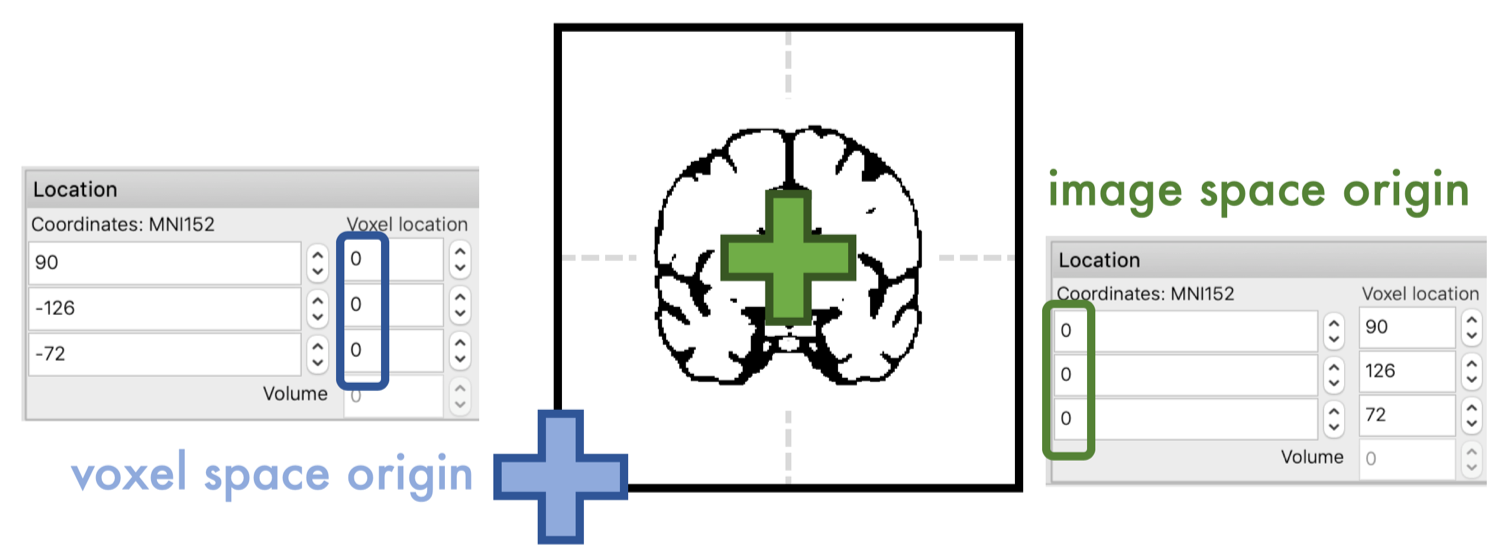
To get the rotation matrix, however, we have to wrap our head around a tricky topic, the coordinate system of the image. Typically, neuroimaging data comes with two coordinate systems that define ‘voxel space’ and ‘image space’. The origin of the voxel space is usually in the ‘left-posterior-inferior’ corner of your image. In image space, the origin is usually placed in the center of the brain. In FSL’s image viewer fsl_eyes, the coordinate for both spaces are displayed.

Coordinate Systems

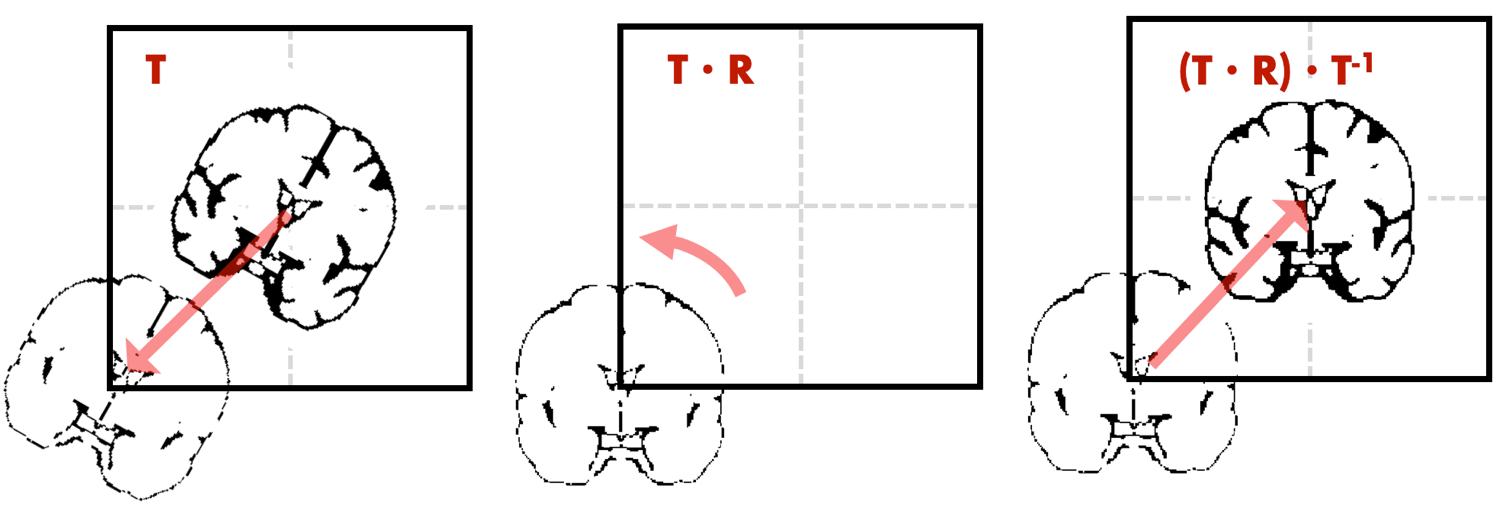
A matrix multiplication as defined above, performed for example by FSL’s ‘applywarp’, will assume that we are rotating around the origin of the voxel space, which is NOT what we want in image alignment. That’s why we first need to compensate for the ‘offset’ between the two coordinate systems. The information about this ‘offset’ is stored in the header of your scan within the ‘sform’ (or ‘qform’). The sform is an affine matrix, where the offset is represented in the last column (I recommend reading: https://fsl.fmrib.ox.ac.uk/fsl/fslwiki/Orientation%20Explained).

That means we require 3 steps to rotate the brain image: 1) translate the image to the voxel space origin using the offset from sform, 2) apply a rotation based on desired angles, 3) translate the image back to the image space origin using the inverse of the offset.

Rotation matrix

Equipped with this theoretical knowledge, we can compose our desired rigid body transformation using a few simple code lines. Working through such a transformation manually helped me a lot to understand how neuroimaging data is stored and displayed and how it can be manipulated outside of the standard processing toolboxes. I hope I could make this topic accessible without going too deep in the maths and below I post some related python snippets.

Thank you for reading this post :-)

Nicole

Code snippets and more details

The following website provides useful comments on translation and rotation: https://www.learnopencv.com/rotation-matrix-to-euler-angles/.

Translation matrix

A translation can be represented as 3x1 vector or as 4x4 matrix. The conversion is straight forward:

# vector to matrix:
translation_vec = np.array([x, y, z])
T = np.array([[1, 0, 0, translation_vec[0]],
              [0, 1, 0, translation_vec[1]],
              [0, 0, 1, translation_vec[2]],
              [0, 0, 0, 1]])

# matrix to vector:
translation_vec = T[0:3,3]

Rotation matrix

A rotation can be described as 3x1 vector (theta) for the rotation along the three spatial axes. Each of the three rotation components can be described by a rotation matrix. The combined rotation matrix is derived as matrix multiplication of the three matrices:

# vector to matrix:

# define rotation vector in radians
theta = np.array([th1, th2, th3])

R_x = np.array([[ 1, 0,                  0                   ],
                [ 0, math.cos(theta[0]), -math.sin(theta[0]) ],
                [ 0, math.sin(theta[0]),  math.cos(theta[0]) ]])

R_y = np.array([[  math.cos(theta[1]), 0, math.sin(theta[1])],
                [  0,                  1,                  0],
                [ -math.sin(theta[1]), 0, math.cos(theta[1])]])

R_z = np.array([[ math.cos(theta[2]), -math.sin(theta[2]), 0],
                [ math.sin(theta[2]),  math.cos(theta[2]), 0],
                [ 0,               0,                      1]])

R = np.dot(R_z, np.dot( R_y, R_x ))

# add fourth column and row to convert 3x3 to 4x4 matrix:
R = np.vstack((R,[0,0,0]))
R = np.hstack((R, np.array([0,0,0,1]).reshape(-1,1)))


# matrix to vector:
# will only work with an invertible matrix
sy = math.sqrt(R[0,0] * R[0,0] + R[1,0] * R[1,0])
is_singular = sy < 1e-4

if not is_singular:
    x = math.atan2(R[2,1], R[2,2])
    y = math.atan2(-R[2,0], sy)
    z = math.atan2(R[1,0], R[0,0])
else:
    x = math.atan2(-R[1,2], R[1,1])
    y = math.atan2(-R[2,0], sy)
    z = 0

theta = np.array([x, y, z])

Compensate for offset

The following lines create a rotation matrix with adjusting for the offset of the coordinate system as described above:

import nibabel as nib
import numpy as np

# define desired rotation vector
theta = np.array([th1, th2, th3])

# load input image
img = nib.load(filename)

# determine sform
aff = img.get_affine()

# get offset from last column
offset = aff[0:3,3]

# convert theta to matrix (see above)
R = angles_to_rotation_matrix(theta)

# convert offset to matrix (see above)
T = vector_to_translation_matrix(offset)

# concatenate translation, rotation and inverse translation:
M = np.dot(np.linalg.inv(T), np.dot(R,T))

Adjust signs in offset

One last note on the offset of the coordinate system: Depending on the scanner settings the origin of your voxel space might be in a different ‘corner’ than the default (left-posterior-inferior). You can find out if this is the case by moving your cursor along the three spatial axis in your image viewer. You need to observe, if the values for the ‘voxel coordinates’ increase as expected from left to right, from posterior to anterior and from inferior to superior (sometimes called the default RAS+ orientation). If the values decrease instead, you can flip the sign using the following lines:

flip_coordinates = [True False False]
offset[flip_coordinates] = -offset[flip_coordinates]

Otherwise, the nibabel library has some useful tools like nib.aff2axcodes to automatically detect the axis orientations.

References

¹ Jenkinson, M., Beckmann, C. F., Behrens, T. E. J., Woolrich, M. W. & Smith, S. M. FSL. NeuroImage 62, 782–790 (2012).